Maths notes (1)

So I started reading a paper about diffusion (the original DDPM paper) and I was quickly out of my depth. I needed a refresher about probabilities, and actually even more basic stuff like exponential and integration. And I thought why not share the notes here! So this blog post is the content of a python notebook about exponential and the normal distribution, exported to markdown with jupyter nbconvert. It’s not deep or anything, just a nice refresher for myself. Kind of a pain to write math formulas and get them displayed in my Jekyll blog but got it working with Mathjax.

import matplotlib.pyplot as plt
import numpy as np

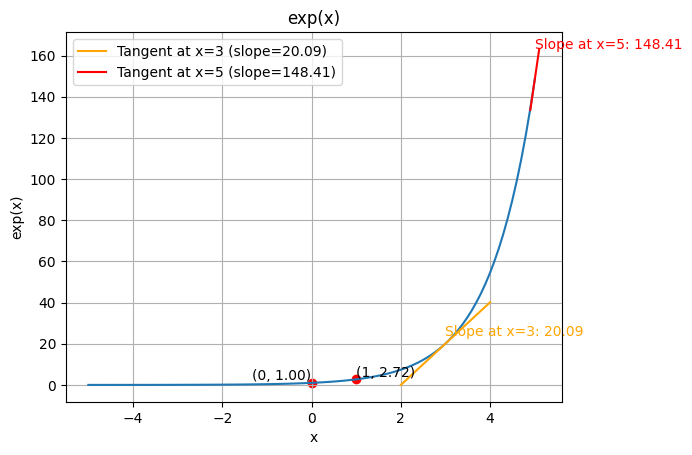
Let’s get started with the exponential: $exp(x) = e^x$.

It’s a function that tends to 0 for $-\infty$ and goes up very quickly as x grows.

There are a few things to know about it :

$e^0 = 1$

$e^1 = e \approx 2.718 $

and the slope (ie the derivative) is the exponential itself ie:

$\frac{d}{dx} e^x = e^x $

Let’s graph it !

import matplotlib.pyplot as plt
import numpy as np

x = np.linspace(-5, 5, 100)
y = np.exp(x)
plt.plot(x, y)

# Values at 0 and 1
plt.scatter([0, 1], [np.exp(0), np.exp(1)], color='red')
plt.text(0, np.exp(0), f"({0}, {np.exp(0):.2f})", fontsize=10, ha='right', va='bottom')
plt.text(1, np.exp(1), f"({1}, {np.exp(1):.2f})", fontsize=10, ha='left', va='bottom')

# Slope at 3 (draw between 2 and 4)
a3 = np.exp(3)
b3 = np.exp(3)
x_tangent3 = np.linspace(2, 4, 50)
y_tangent3 = a3 * (x_tangent3 - 3) + b3
plt.plot(x_tangent3, y_tangent3, color='orange', label=f'Tangent at x=3 (slope={a3:.2f})')
plt.text(3, a3*0.2 + b3, f"Slope at x=3: {a3:.2f}", color='orange', fontsize=10)

# Slope at 5 (draw between 4.9 and 5.1)
a5 = np.exp(5)
b5 = np.exp(5)
x_tangent5 = np.linspace(4.9, 5.1, 50)
y_tangent5 = a5 * (x_tangent5 - 5) + b5
plt.plot(x_tangent5, y_tangent5, color='red', label=f'Tangent at x=5 (slope={a5:.2f})')
plt.text(5, a5*0.1 + b5, f"Slope at x=5: {a5:.2f}", color='red', fontsize=10)

# extra design options
plt.title("exp(x)")
plt.xlabel("x")
plt.ylabel("exp(x)")
plt.grid(True)
plt.legend()
plt.show()

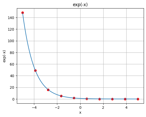
OK now what about the negative $e^{-x}$ ? It’s the same as $1/e^x$ and it’s used as a decay.

x = np.linspace(-5, 5, 100)
y = np.exp(-x)
plt.plot(x, y)

x_reciprocal = np.linspace(-5, 5, 10)
y_reciprocal = 1 / np.exp(x_reciprocal)
plt.scatter(x_reciprocal, y_reciprocal, color='red')

plt.title("exp(-x)")
plt.xlabel("x")
plt.ylabel("exp(-x)")
plt.grid(True)
plt.show()

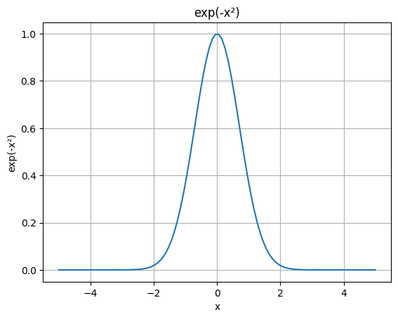
Now in probabilities, to make the nice bell shape we use $e^{-x^2}$. The “square” part is to make $x$ always positive (so we have the symmetry about zero or whatever mean we want, the “$\mu$” in the Gaussian formula) and the “minus” ensures the decay.

x = np.linspace(-5, 5, 100)
y = np.exp(-(x ** 2))
plt.plot(x, y)

plt.title("exp(-x²)")
plt.xlabel("x")
plt.ylabel("exp(-x²)")
plt.grid(True)
plt.show()

Now, the Gaussian integral $ I = \int_{-\infty}^{\infty} e^{-x^2} \, dx$ can be shown to be equal to $\sqrt \pi$ (the trick is to compute $I^2$ and then to switch to polar coordinate etc etc).

From here we can define the PDF (Probability Density Function) that will have an integral of 1 thanks to a normalization factor :

\[\phi(z) = \frac{1}{\sqrt{2\pi}} e^{-z^2 / 2}\]

So it’s like the normal distribution $\mathcal{N}$ with variance of 1 and mean of 0.

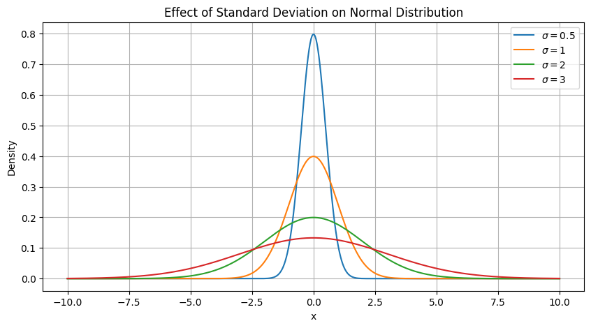
The mean is written “mu” ($\mu$) and the standard deviation is sigma ($\sigma$) (it measures the spread), and the variance is $\sigma^2$. Let’s draw it for various sigmas !

import numpy as np
import matplotlib.pyplot as plt

x = np.linspace(-10, 10, 500)
mu = 0
sigmas = [0.5, 1, 2, 3]  # Various standard deviations

plt.figure(figsize=(10, 5))

for sigma in sigmas:
    y = (1 / (sigma * np.sqrt(2 * np.pi))) * np.exp(-(x - mu)**2 / (2*sigma**2))
    plt.plot(x, y, label=fr'$\sigma={sigma}$')

plt.title("Effect of Standard Deviation on Normal Distribution")
plt.xlabel("x")
plt.ylabel("Density")
plt.grid(True)
plt.legend()
plt.show()

Now we can check that the probability for a value to be within the first sigma is around 68%.

mu = 0
sigma = 1

# Define the standard normal PDF
def pdf(x):
    return (1 / np.sqrt(2 * np.pi)) * np.exp(-(x - mu)**2 / (2 * sigma**2))

# Create x values in the 1σ range
x = np.linspace(mu - sigma, mu + sigma, 1000)  # dense for accuracy
y = pdf(x)

# Approximate the integral using the trapezoidal rule
prob_1sigma = np.trapezoid(y, x)

print("Approximate probability in 1σ region:", prob_1sigma)

Approximate probability in 1σ region: 0.6826893305001358

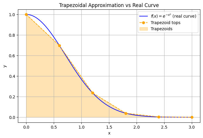
Wait, trapezoidal rule ? It’s a numerical method of integration, let’s see how it looks.

# Few points for trapezoidal approximation
x_coarse = np.linspace(0, 3, 6)        # only 6 points
y_coarse = np.exp(-x_coarse**2)

# Smooth curve for the real function
x_fine = np.linspace(0, 3, 500)
y_fine = np.exp(-x_fine**2)

# Approximate area using trapezoidal rule
area_approx = np.trapezoid(y_coarse, x_coarse)
print("Approx area:", area_approx)

# Plot smooth curve
plt.figure(figsize=(8,5))
plt.plot(x_fine, y_fine, 'b-', label=r'$f(x)=e^{-x^2}$ (real curve)')

# Plot trapezoidal approximation
plt.plot(x_coarse, y_coarse, 'o--', color='orange', label='Trapezoid tops')
plt.fill_between(x_coarse, 0, y_coarse, alpha=0.3, color='orange', label='Trapezoids')

plt.title("Trapezoidal Approximation vs Real Curve")
plt.xlabel("x")
plt.ylabel("y")
plt.legend()
plt.grid(True)
plt.show()

Approx area: 0.8861884778115766

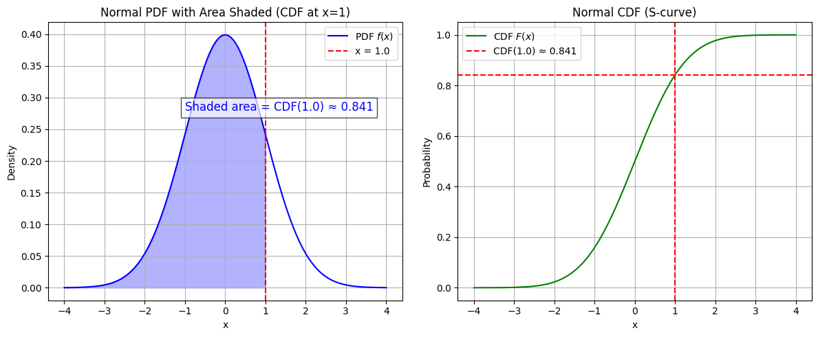
Oook so we have the PDF, but if we want the probability at a given point we want the Cumulative Distribution function (CDF). It’s the integral of the PDF (the area from $-\infty$ to $x$)

import numpy as np
import matplotlib.pyplot as plt
import math

# --- PDF and CDF definitions ---
def normal_pdf(x, mu=0, sigma=1):
    return (1 / (sigma * np.sqrt(2 * np.pi))) * np.exp(-(x - mu)**2 / (2*sigma**2))

def normal_cdf_exact(x, mu=0, sigma=1):
    z = (x - mu) / (sigma * np.sqrt(2))
    return 0.5 * (1 + math.erf(z))

# --- Visualization parameters ---
mu, sigma = 0, 1
x = np.linspace(-4, 4, 500)
pdf = normal_pdf(x, mu, sigma)
cdf = [normal_cdf_exact(xi, mu, sigma) for xi in x]

# Pick a point to visualize CDF
x0 = 1.0
cdf_val = normal_cdf_exact(x0, mu, sigma)

plt.figure(figsize=(12,5))

# --- Left: PDF ---
plt.subplot(1,2,1)
plt.plot(x, pdf, label='PDF $f(x)$', color='blue')
plt.fill_between(x, 0, pdf, where=(x <= x0), color='blue', alpha=0.3)
plt.axvline(x0, color='red', linestyle='--', label=f'x = {x0}')
plt.title("Normal PDF with Area Shaded (CDF at x=1)")
plt.xlabel("x")
plt.ylabel("Density")
plt.legend()
plt.grid(True)
# Annotate the shaded area with the CDF value
plt.text(
    x0 - 2, max(pdf)*0.7,
    f"Shaded area = CDF({x0}) ≈ {cdf_val:.3f}",
    fontsize=12, color='blue', bbox=dict(facecolor='white', alpha=0.7)
)

# --- Right: CDF ---
plt.subplot(1,2,2)
plt.plot(x, cdf, label='CDF $F(x)$', color='green')
plt.axhline(cdf_val, color='red', linestyle='--', label=f'CDF({x0:.1f}) ≈ {cdf_val:.3f}')
plt.axvline(x0, color='red', linestyle='--')
plt.title("Normal CDF (S-curve)")
plt.xlabel("x")
plt.ylabel("Probability")
plt.legend()
plt.grid(True)

plt.tight_layout()

At that point I kind of forgot what I was looking for in the first place, so I should just go back to the paper and try to make some progress in it.