So I started reading a paper about diffusion (the original DDPM paper) and I was quickly out of my depth. I needed a refresher about probabilities, and actually even more basic stuff like exponential and integration. And I thought why not share the notes here! So this blog post is the content of a python notebook about exponential and the normal distribution, exported to markdown with jupyter nbconvert. It’s not deep or anything, just a nice refresher for myself. Kind of a pain to write math formulas and get them displayed in my Jekyll blog but got it working with Mathjax.
1
2
| import matplotlib.pyplot as plt
import numpy as np
|
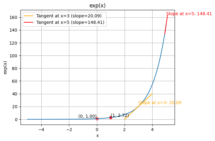
Let’s get started with the exponential: $exp(x) = e^x$.
It’s a function that tends to 0 for $-\infty$ and goes up very quickly as x grows.
There are a few things to know about it :
$e^0 = 1$
$e^1 = e \approx 2.718 $
and the slope (ie the derivative) is the exponential itself ie:
$\frac{d}{dx} e^x = e^x $
Let’s graph it !
 1
 2
 3
 4
 5
 6
 7
 8
 9
10
11
12
13
14
15
16
17
18
19
20
21
22
23
24
25
26
27
28
29
30
31
32
33
34
35
| import matplotlib.pyplot as plt
import numpy as np
x = np.linspace(-5, 5, 100)
y = np.exp(x)
plt.plot(x, y)
# Values at 0 and 1
plt.scatter([0, 1], [np.exp(0), np.exp(1)], color='red')
plt.text(0, np.exp(0), f"({0}, {np.exp(0):.2f})", fontsize=10, ha='right', va='bottom')
plt.text(1, np.exp(1), f"({1}, {np.exp(1):.2f})", fontsize=10, ha='left', va='bottom')
# Slope at 3 (draw between 2 and 4)
a3 = np.exp(3)
b3 = np.exp(3)
x_tangent3 = np.linspace(2, 4, 50)
y_tangent3 = a3 * (x_tangent3 - 3) + b3
plt.plot(x_tangent3, y_tangent3, color='orange', label=f'Tangent at x=3 (slope={a3:.2f})')
plt.text(3, a3*0.2 + b3, f"Slope at x=3: {a3:.2f}", color='orange', fontsize=10)
# Slope at 5 (draw between 4.9 and 5.1)
a5 = np.exp(5)
b5 = np.exp(5)
x_tangent5 = np.linspace(4.9, 5.1, 50)
y_tangent5 = a5 * (x_tangent5 - 5) + b5
plt.plot(x_tangent5, y_tangent5, color='red', label=f'Tangent at x=5 (slope={a5:.2f})')
plt.text(5, a5*0.1 + b5, f"Slope at x=5: {a5:.2f}", color='red', fontsize=10)
# extra design options
plt.title("exp(x)")
plt.xlabel("x")
plt.ylabel("exp(x)")
plt.grid(True)
plt.legend()
plt.show()
|
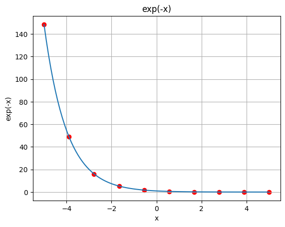
OK now what about the negative $e^{-x}$ ? It’s the same as $1/e^x$ and it’s used as a decay.
 1
 2
 3
 4
 5
 6
 7
 8
 9
10
11
12
13
| x = np.linspace(-5, 5, 100)
y = np.exp(-x)
plt.plot(x, y)
x_reciprocal = np.linspace(-5, 5, 10)
y_reciprocal = 1 / np.exp(x_reciprocal)
plt.scatter(x_reciprocal, y_reciprocal, color='red')
plt.title("exp(-x)")
plt.xlabel("x")
plt.ylabel("exp(-x)")
plt.grid(True)
plt.show()
|
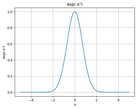
Now in probabilities, to make the nice bell shape we use $e^{-x^2}$. The “square” part is to make $x$ always positive (so we have the symmetry about zero or whatever mean we want, the “$\mu$” in the Gaussian formula) and the “minus” ensures the decay.
1
2
3
4
5
6
7
8
9
| x = np.linspace(-5, 5, 100)
y = np.exp(-(x ** 2))
plt.plot(x, y)
plt.title("exp(-x²)")
plt.xlabel("x")
plt.ylabel("exp(-x²)")
plt.grid(True)
plt.show()
|
Now, the Gaussian integral $ I = \int_{-\infty}^{\infty} e^{-x^2} , dx$ can be shown to be equal to $\sqrt \pi$ (the trick is to compute $I^2$ and then to switch to polar coordinate etc etc).
From here we can define the PDF (Probability Density Function) that will have an integral of 1 thanks to a normalization factor :
$$\phi(z) = \frac{1}{\sqrt{2\pi}} e^{-z^2 / 2}$$
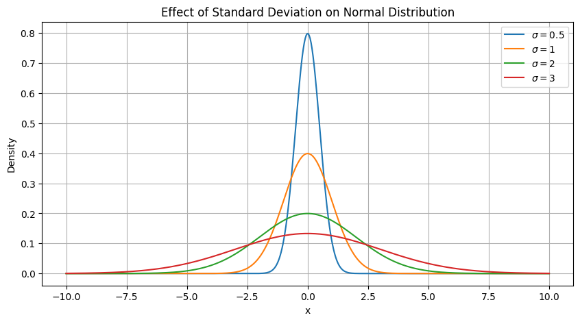
So it’s like the normal distribution $\mathcal{N}$ with variance of 1 and mean of 0.
The mean is written “mu” ($\mu$) and the standard deviation is sigma ($\sigma$) (it measures the spread), and the variance is $\sigma^2$. Let’s draw it for various sigmas !
 1
 2
 3
 4
 5
 6
 7
 8
 9
10
11
12
13
14
15
16
17
18
19
| import numpy as np
import matplotlib.pyplot as plt
x = np.linspace(-10, 10, 500)
mu = 0
sigmas = [0.5, 1, 2, 3] # Various standard deviations
plt.figure(figsize=(10, 5))
for sigma in sigmas:
y = (1 / (sigma * np.sqrt(2 * np.pi))) * np.exp(-(x - mu)**2 / (2*sigma**2))
plt.plot(x, y, label=fr'$\sigma={sigma}$')
plt.title("Effect of Standard Deviation on Normal Distribution")
plt.xlabel("x")
plt.ylabel("Density")
plt.grid(True)
plt.legend()
plt.show()
|
Now we can check that the probability for a value to be within the first sigma is around 68%.
 1
 2
 3
 4
 5
 6
 7
 8
 9
10
11
12
13
14
15
| mu = 0
sigma = 1
# Define the standard normal PDF
def pdf(x):
return (1 / np.sqrt(2 * np.pi)) * np.exp(-(x - mu)**2 / (2 * sigma**2))
# Create x values in the 1σ range
x = np.linspace(mu - sigma, mu + sigma, 1000) # dense for accuracy
y = pdf(x)
# Approximate the integral using the trapezoidal rule
prob_1sigma = np.trapezoid(y, x)
print("Approximate probability in 1σ region:", prob_1sigma)
|
Approximate probability in 1σ region: 0.6826893305001358
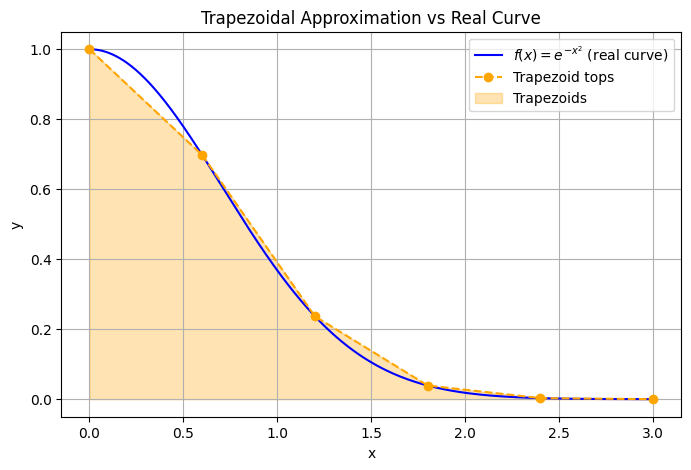
Wait, trapezoidal rule ? It’s a numerical method of integration, let’s see how it looks.
 1
 2
 3
 4
 5
 6
 7
 8
 9
10
11
12
13
14
15
16
17
18
19
20
21
22
23
24
25
26
| # Few points for trapezoidal approximation
x_coarse = np.linspace(0, 3, 6) # only 6 points
y_coarse = np.exp(-x_coarse**2)
# Smooth curve for the real function
x_fine = np.linspace(0, 3, 500)
y_fine = np.exp(-x_fine**2)
# Approximate area using trapezoidal rule
area_approx = np.trapezoid(y_coarse, x_coarse)
print("Approx area:", area_approx)
# Plot smooth curve
plt.figure(figsize=(8,5))
plt.plot(x_fine, y_fine, 'b-', label=r'$f(x)=e^{-x^2}$ (real curve)')
# Plot trapezoidal approximation
plt.plot(x_coarse, y_coarse, 'o--', color='orange', label='Trapezoid tops')
plt.fill_between(x_coarse, 0, y_coarse, alpha=0.3, color='orange', label='Trapezoids')
plt.title("Trapezoidal Approximation vs Real Curve")
plt.xlabel("x")
plt.ylabel("y")
plt.legend()
plt.grid(True)
plt.show()
|
Approx area: 0.8861884778115766
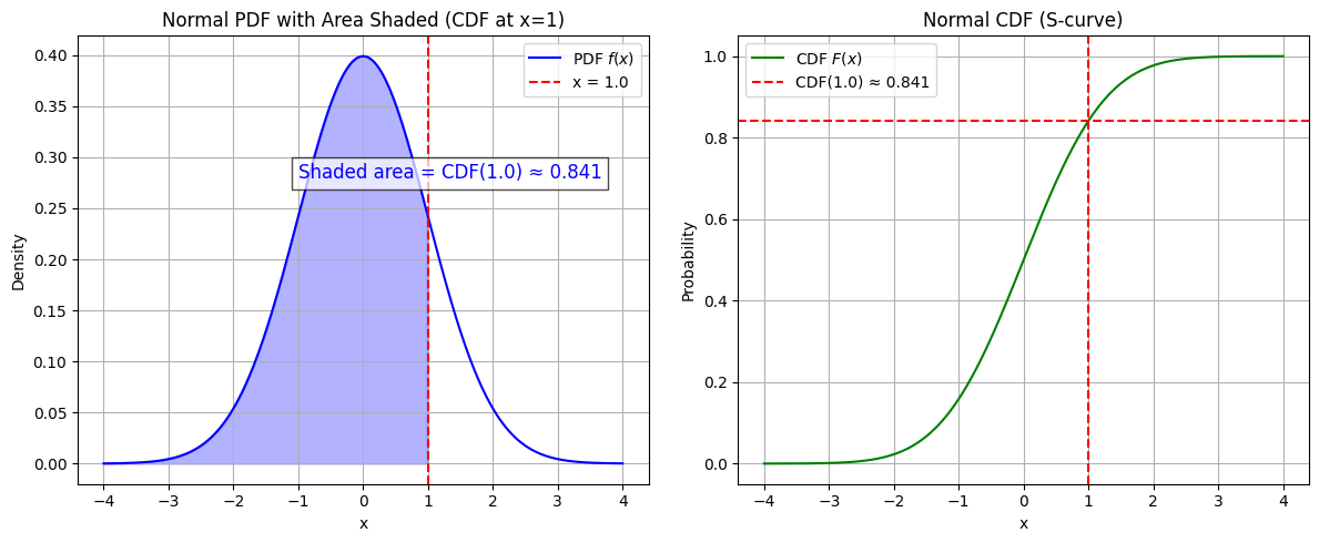
Oook so we have the PDF, but if we want the probability at a given point we want the Cumulative Distribution function (CDF). It’s the integral of the PDF (the area from $-\infty$ to $x$)
 1
 2
 3
 4
 5
 6
 7
 8
 9
10
11
12
13
14
15
16
17
18
19
20
21
22
23
24
25
26
27
28
29
30
31
32
33
34
35
36
37
38
39
40
41
42
43
44
45
46
47
48
49
50
51
52
53
| import numpy as np
import matplotlib.pyplot as plt
import math
# --- PDF and CDF definitions ---
def normal_pdf(x, mu=0, sigma=1):
return (1 / (sigma * np.sqrt(2 * np.pi))) * np.exp(-(x - mu)**2 / (2*sigma**2))
def normal_cdf_exact(x, mu=0, sigma=1):
z = (x - mu) / (sigma * np.sqrt(2))
return 0.5 * (1 + math.erf(z))
# --- Visualization parameters ---
mu, sigma = 0, 1
x = np.linspace(-4, 4, 500)
pdf = normal_pdf(x, mu, sigma)
cdf = [normal_cdf_exact(xi, mu, sigma) for xi in x]
# Pick a point to visualize CDF
x0 = 1.0
cdf_val = normal_cdf_exact(x0, mu, sigma)
plt.figure(figsize=(12,5))
# --- Left: PDF ---
plt.subplot(1,2,1)
plt.plot(x, pdf, label='PDF $f(x)$', color='blue')
plt.fill_between(x, 0, pdf, where=(x <= x0), color='blue', alpha=0.3)
plt.axvline(x0, color='red', linestyle='--', label=f'x = {x0}')
plt.title("Normal PDF with Area Shaded (CDF at x=1)")
plt.xlabel("x")
plt.ylabel("Density")
plt.legend()
plt.grid(True)
# Annotate the shaded area with the CDF value
plt.text(
x0 - 2, max(pdf)*0.7,
f"Shaded area = CDF({x0}) ≈ {cdf_val:.3f}",
fontsize=12, color='blue', bbox=dict(facecolor='white', alpha=0.7)
)
# --- Right: CDF ---
plt.subplot(1,2,2)
plt.plot(x, cdf, label='CDF $F(x)$', color='green')
plt.axhline(cdf_val, color='red', linestyle='--', label=f'CDF({x0:.1f}) ≈ {cdf_val:.3f}')
plt.axvline(x0, color='red', linestyle='--')
plt.title("Normal CDF (S-curve)")
plt.xlabel("x")
plt.ylabel("Probability")
plt.legend()
plt.grid(True)
plt.tight_layout()
|
At that point I kind of forgot what I was looking for in the first place, so I should just go back to the paper and try to make some progress in it.